A Framework for Consistently Smooth and Responsive Flight Control via Reinforcement Learning
Abstract
We focus on the problem of reliably training Reinforcement Learning (RL) models (agents) for stable low-level control in embedded systems and test our methods on a high-performance, custom-built quadrotor platform. A common but often under-studied problem in developing RL agents for continuous control is that the control policies developed are not always smooth. This lack of smoothness can be a major problem when learning controllers intended for deployment on real hardware as it can result in control instability and hardware failure.
Issues of noisy control are further accentuated when training RL agents in simulation due to simulators ultimately being imperfect representations of reality – what is known as the reality gap. To combat issues of instability in RL agents, we propose a systematic framework, `REinforcement-based transferable Agents through Learning’ (RE+AL), for designing simulated training environments which preserve the quality of trained agents when transferred to real platforms. RE+AL is an evolution of the Neuroflight infrastructure detailed in technical reports prepared by members of our research group. Neuroflight is a state-of-the-art framework for training RL agents for low-level attitude control. RE+AL improves and completes Neuroflight by solving a number of important limitations that hindered the deployment of Neuroflight to real hardware. We benchmark RE+AL on the NF1 racing quadrotor developed as part of Neuroflight. We demonstrate that RE+AL significantly mitigates the previously observed issues of smoothness in RL agents. Additionally, RE+AL is shown to consistently train agents that are flight-capable and with minimal degradation in controller quality upon transfer. RE+AL agents also learn to perform better than a tuned PID controller, with better tracking errors, smoother control and reduced power consumption.
Main Results
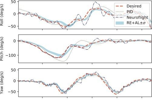
This is a comparison of how well Neuroflight and RE+AL follow the Desired trajectories in simulation compared to PID controllers. Notice how PID tends to drift off the Desired line incurring more error than Neuroflight or RE+AL
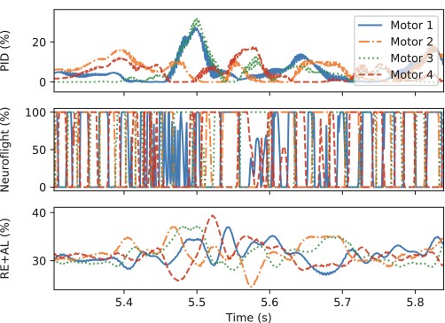
However Neuroflight‘s motor usage to achieve that trajectory is quite erradic, RE+AL on the other hand smoothly adjusts its motor values without being sensitive to noise in the gyroscope readings.
We then took a Fourier transform of motor outputs during actual flights and plotted them to show how RE+AL compares to Neuroflight:
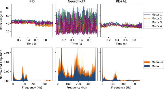
In short, our method allowed for very significant gains in motor actuation smoothness, leading to agents drawing, on average, 5.86±3.10 amps during flight tests, while the Neuroflight agents drew an average of 22.87 amps on similar tests. PID meanwhile took an average of 8.07 amps.
Contributions
Goal Generation
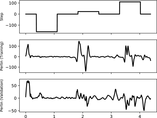
We reworked the Reinforcement Learning environment so that control inputs are more realistic (Perlin noise based vs a step-wise function). This allowed for the agent to constantly try following a trajectory, rather than follow a bit and then wait.
Reward Composition
We then focused on reward engineering, we noticed that the classical techniques for composing reward signals causes many issues in terms of hyper-parameter sensitivity and the algorithms being stuck in local-minima. Usually the signals are summed up and weights are tweaked according to learned behavior seen after training for a while, it looks like this:
| \begin{equation} r_t = \sum _k^K w_k r_k \end{equation} |
We instead proposed to normalize reward signals and then “multiplicatively” compose them, the full equation being the following:
| \begin{equation} r_t = g(r) = \left(\prod ^K_k \min (1,r_k+\epsilon)\right)^{K^{-1}}\end{equation} |
This allowed us to go from Neuroflight’s individual reward components which are the following:
| \begin{align} r_a &= -100 \cdot \max _i\left(\left|y_{t}^{(i)} – y_{t-1}^{(i)}\right|\right) \end{align} |
| \begin{align} r_b &= 1000 \cdot \left(1 – \frac{1}{4}\sum _i y_t^{(i)}\right){1\!\!1}_{{\bf e}_t \lt \epsilon } \end{align} |
| \begin{align} r_e &= ||{\bf e}_{t-1}|| – ||{\bf e}_{t}|| \end{align} |
| \begin{align} r_o &= -1\times 10^9 \cdot \sum _i \max \left(y_{t}^{(i)} – 1, 0\right) \end{align} |
| \begin{align} r_n &= -1\times 10^9 \cdot {1\!\!1}_{||{\bf \bar{\phi }}_t|| \gt 0} \cdot \sum _i {1\!\!1}_{y_t^{(i)} = 0} , \end{align} |
To our reward signals which are much simpler:
| \begin{equation} p_s = || \phi _t – \bar{\phi }_t ||_4 \end{equation} |
| \begin{equation} p_c^{(i)} = \big |y^{(i)}_t – y^{(i)}_{t-1}\big | \end{equation} |
| \begin{equation} p_u^{(i)} = \big |y^{(i)}_t – \mu \big | \end{equation} |
We then tried our technique on many standard Reinforcement Learning benchmark tasks and observed greater than 50% lower reward variance on 19/24 tasks. And trained agents consistently satisfied our intended goals, rather than having a good reward and unintended behavior as was observed with the standard reward structure in those environments.